机器学习大作业

1. 赛题理解

1.1 赛题概况：

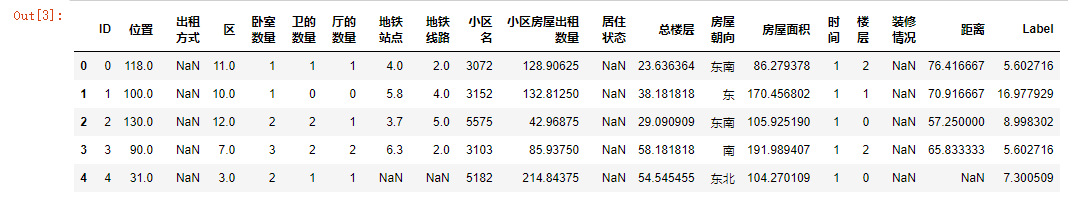
给定房屋租金价格的各个影响因素数据，建立模型预测国内某城市房屋的租金价格。

1.2 数据概况：

（1）ID：编号；
（2）时间：房屋信息采集的时间；
（3）小区名：房屋所在小区，已脱敏处理；
（4）小区房屋出租数量：小区出租房屋数量，已脱敏处理；
（5）楼层：0、1、2分别表示楼层低，中，高；
（6）总层数：房屋所在建筑的总楼层数，已脱敏处理；
（7）房屋面积：房屋面积数值，已脱敏处理；
（8）房屋朝向：房屋的朝向；
（9）居住状态：房屋的居住状态，表示是否已出租或居住中，已脱敏处理；
（10）卧室数量：户型信息，数字表示卧室的个数；
（11）卫的数量：户型信息，数字表示卫生间的个数；
（12）厅的数量：户型信息，数字表示厅的个数；
（13）出租方式：是否整租，1为整租，0为合租；
（14）区：房屋所在的区级行政单位，用数字表示；
（15）位置：小区所在商圈位置，已脱敏处理；
（16）地铁线路:数字表示第几条线路，已脱敏处理；
（17）地铁站点房屋临近的地铁站，脱敏处理;
（18）距离：房屋距地铁站距离，脱敏处理;
（19）装修情况：房屋的装修档次，数值越高表示装修档次越高，脱敏处理;
（20）Label：月租金，标签值，脱敏处理。

1.3 预测指标：

通过计算MSE来衡量回归模型的优劣。MSE越小，说明回归模型越好。
评分算法参考代码如下：

from sklearn.metrics import mean_squared_error
y_true = [1, 2, 3, 4] 
y_pred = [1.1, 2.2, 3.3, 4.4]
score = mean_squared_error(y_true, y_pred)

1.4 赛题分析：

由于多数特征与Label之间的相关性不强，应考虑从原始数据中构建新的特征，以此来优化模型。

2. 数据分析

2.1 载入数据

# 载入库
import pandas as pd
import numpy as np
from numpy import nan as NaN
import matplotlib.pyplot as plt
plt.rcParams['font.sans-serif']=['SimHei']
plt.rcParams['axes.unicode_minus']=False
import seaborn as sns
import warnings
warnings.filterwarnings('ignore')

from sklearn import linear_model
import lightgbm as lgb
import xgboost as xgb
import catboost as cb
from sklearn.model_selection import train_test_split,GridSearchCV,cross_val_score
from sklearn.metrics import mean_squared_error,make_scorer

1
2
3

# 载入数据
train = pd.read_csv("train.csv")
test = pd.read_csv("test_noLabel.csv")

1 2	`# 查看训练集 train.head()`

1 2	`# 查看测试集 test.head()`

2.2 判断异常数据

# 查看训练集和测试集数据大小、数据类型、缺失情况等信息
train.info()
print('-------------------')
test.info()

<class 'pandas.core.frame.DataFrame'>
RangeIndex: 196539 entries, 0 to 196538
Data columns (total 20 columns):
 #   Column    Non-Null Count   Dtype  
---  ------    --------------   -----  
 0   ID        196539 non-null  int64  
 1   位置        196508 non-null  float64
 2   出租方式      24230 non-null   float64
 3   区         196508 non-null  float64
 4   卧室数量      196539 non-null  int64  
 5   卫的数量      196539 non-null  int64  
 6   厅的数量      196539 non-null  int64  
 7   地铁站点      91778 non-null   float64
 8   地铁线路      91778 non-null   float64
 9   小区名       196539 non-null  int64  
 10  小区房屋出租数量  195538 non-null  float64
 11  居住状态      20138 non-null   float64
 12  总楼层       196539 non-null  float64
 13  房屋朝向      196539 non-null  object 
 14  房屋面积      196539 non-null  float64
 15  时间        196539 non-null  int64  
 16  楼层        196539 non-null  int64  
 17  装修情况      18492 non-null   float64
 18  距离        91778 non-null   float64
 19  Label     196539 non-null  float64
dtypes: float64(12), int64(7), object(1)
memory usage: 30.0+ MB
-------------------
<class 'pandas.core.frame.DataFrame'>
RangeIndex: 56279 entries, 0 to 56278
Data columns (total 19 columns):
 #   Column    Non-Null Count  Dtype  
---  ------    --------------  -----  
 0   ID        56279 non-null  int64  
 1   位置        56269 non-null  float64
 2   出租方式      4971 non-null   float64
 3   区         56269 non-null  float64
 4   卧室数量      56279 non-null  int64  
 5   卫的数量      56279 non-null  int64  
 6   厅的数量      56279 non-null  int64  
 7   地铁站点      26494 non-null  float64
 8   地铁线路      26494 non-null  float64
 9   小区名       56279 non-null  int64  
 10  小区房屋出租数量  56257 non-null  float64
 11  居住状态      4483 non-null   float64
 12  总楼层       56279 non-null  float64
 13  房屋朝向      56279 non-null  object 
 14  房屋面积      56279 non-null  float64
 15  时间        56279 non-null  int64  
 16  楼层        56279 non-null  int64  
 17  装修情况      4207 non-null   float64
 18  距离        26494 non-null  float64
dtypes: float64(11), int64(7), object(1)
memory usage: 8.2+ MB

# 查看训练集具体缺失百分比
train_missing = (train.isnull().sum()/len(train))*100
train_missing = train_missing.drop(train_missing[train_missing==0].index).sort_values(ascending=False)
train_missing

装修情况        90.591180
居住状态        89.753688
出租方式        87.671658
地铁站点        53.302907
地铁线路        53.302907
距离          53.302907
小区房屋出租数量     0.509314
位置           0.015773
区            0.015773
dtype: float64

# 查看测试集具体缺失百分比
test_missing = (test.isnull().sum()/len(test))*100
test_missing = test_missing.drop(test_missing[test_missing==0].index).sort_values(ascending=False)
test_missing

装修情况        92.524743
居住状态        92.034329
出租方式        91.167220
地铁站点        52.923826
地铁线路        52.923826
距离          52.923826
小区房屋出租数量     0.039091
位置           0.017769
区            0.017769
dtype: float64

2.3 数据分布及相关性分析

1	`sns.histplot(train['Label'], kde=True)`

# 查看相关性
columns = train.columns.drop('ID')
correlation = train[columns].corr()
plt.figure(figsize=(20, 10)) 
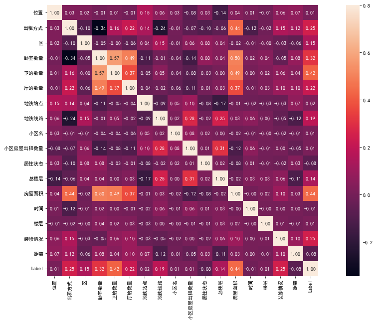
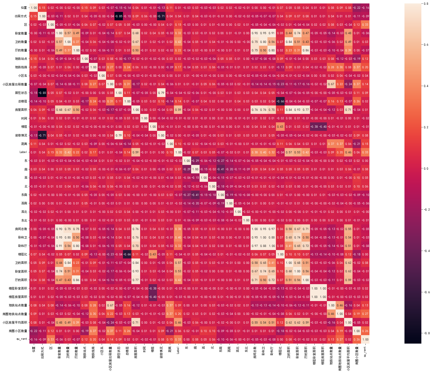
sns.heatmap(correlation,square = True, annot=True, fmt='0.2f',vmax=0.8)

通过相关性分析可以看出，房屋面积、卫的数量、卧室数量、厅的数量和租金之间相关性最高，其次是出租方式、装修情况、地铁线路、区、总楼层，其他特征相关性比较低。

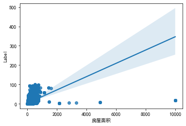
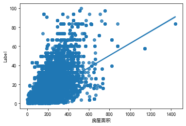
1 2	`# 房屋面积 sns.regplot(x=train['房屋面积'],y=train['Label'])`

从图中可以看出房屋面积数据中存在异常点，因为测试集上房屋的最大面积为1441.576，则将删除阈值选为1441.576，下面将异常点删除：

1
2
3

# 删除异常值
train = train.drop(train[train['房屋面积']>1441.576].index)
sns.regplot(x=train['房屋面积'],y=train['Label'])

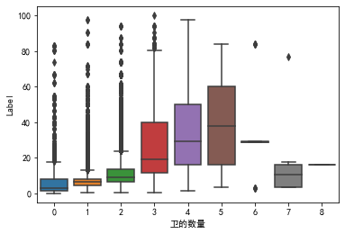
因为接下来的卫的数量、卧室数量、厅的数量属于离散型数据，所以采用箱线图来观察。

1 2	`# 卫的数量 sns.boxplot(x=train['卫的数量'],y=train['Label'])`

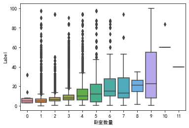
1 2	`# 卧室数量 sns.boxplot(x=train['卧室数量'],y=train['Label'])`

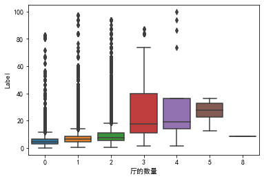
1 2	`# 厅的数量 sns.boxplot(x=train['厅的数量'],y=train['Label'])`

3. 特征工程

3.1 离散化编码处理

# 对object类型的特征“房屋朝向”进行离散化编码处理
orientation_headers = ['东', '南', '西', '北',
                       '东南', '西南', '西北', '东北']
def fill_orientation(item, orientation):
    x = item.split(' ')
    return 1 if orientation in x else 0
 
for i in orientation_headers:
    train[i] = train['房屋朝向'].apply(lambda x: fill_orientation(x, i))

for i in orientation_headers:
    test[i] = test['房屋朝向'].apply(lambda x: fill_orientation(x, i))
    
train.drop('房屋朝向', axis=1, inplace=True)
test.drop('房屋朝向', axis=1, inplace=True)

3.2 缺失值处理

上文去除了房屋面积的异常值，接下来进行缺失值处理

# 发现数据是连续的，但其中缺少5，可能是数据输入遗漏掉了，因此填充缺失值为5
train['区'] = train['区'].fillna(5)
test['区'] = test['区'].fillna(5)
# 位置中缺少76，同理填充缺失值为76
train['位置'] = train['位置'].fillna(76)
test['位置'] = test['位置'].fillna(76)

# 进行排序后，使用前一条数据对小区房屋出租数量进行填充
train = train.sort_values(by=['区','小区名', '楼层',], ascending=(True, True, True))
test = test.sort_values(by=['区','小区名', '楼层'], ascending=(True, True, True))

train['小区房屋出租数量'] = train['小区房屋出租数量'].fillna(method='pad')
test['小区房屋出租数量'] = test['小区房屋出租数量'].fillna(method='pad')

data = pd.concat([train, test], axis=0, ignore_index=True)

# 使用小区房屋与地铁站的平均距离对同一小区房屋到地铁站距离进行填充
xiaoqu_dis = data.groupby('小区名')['距离'].mean()
dict_xiaoqu_dis = {'小区名':xiaoqu_dis.index,'平均距离':xiaoqu_dis.values}
df_xiaoqu_dis = pd.DataFrame(dict_xiaoqu_dis)

data = data.merge(df_xiaoqu_dis, on='小区名',how='left')
data['距离'] = data['距离'].fillna(data['平均距离'])

# 用小区地铁线路填充同一小区地铁新路的缺失值
xiaoqu_sub_line = data.groupby('小区名')['地铁线路'].max()
dict_xiaoqu_sub_line = {'小区名':xiaoqu_sub_line.index,'小区地铁线路':xiaoqu_sub_line.values}
df_xiaoqu_sub_line = pd.DataFrame(dict_xiaoqu_sub_line)

data = data.merge(df_xiaoqu_sub_line, on='小区名',how='left')
data['地铁线路'] = data['小区地铁线路']

# 用小区地铁站点填充同一小区地铁站点的缺失值
xiaoqu_sub = data.groupby('小区名')['地铁站点'].max()
dict_xiaoqu_sub = {'小区名':xiaoqu_sub.index,'小区地铁站点':xiaoqu_sub.values}
df_xiaoqu_sub = pd.DataFrame(dict_xiaoqu_sub)

data = data.merge(df_xiaoqu_sub, on='小区名',how='left')
data['地铁站点'] = data['小区地铁站点']

data.drop(['平均距离','小区地铁线路','小区地铁站点'],axis=1,inplace=True)

# 对其他缺失值进行固定值填充
data['距离'] = data['距离'].fillna(0)
data['居住状态'] = data['居住状态'].fillna(0)
data['装修情况'] = data['装修情况'].fillna(0)
data['出租方式'] = data['出租方式'].fillna(2)

# 构造新的特征
data['房间总数'] = data['卫的数量'] + data['卧室数量'] + data['厅的数量']
data['卧和卫'] = data['卫的数量'] + data['卧室数量']
data['卧和厅'] = data['卧室数量'] + data['厅的数量']

data['楼层比'] = (data['楼层'] + 1) / data['总楼层']

data['卫的面积'] = data['房屋面积']*(data['卫的数量']/data['房间总数'])
data['卧室面积'] = data['房屋面积']*(data['卧室数量']/data['房间总数'])
data['厅的面积'] = data['房屋面积']*(data['厅的数量']/data['房间总数'])

# 每个楼层的卧室面积
temp = data.groupby('楼层')['卧室面积'].sum().reset_index()
temp.columns = ['楼层','楼层卧室面积']
data = data.merge(temp, how = 'left',on = '楼层')

# 每个楼层的房屋面积
temp = data.groupby('楼层')['房屋面积'].sum().reset_index()
temp.columns = ['楼层','楼层房屋面积']
data = data.merge(temp, how = 'left',on = '楼层')

# 每个小区附近的地铁站点数
temp = data.groupby('小区名')['地铁站点'].count().reset_index()
temp.columns = ['小区名','地铁站点数量']
data = data.merge(temp, how = 'left',on = '小区名')

# 每个位置附近的地铁站点数
temp = data.groupby('位置')['地铁站点'].count().reset_index()
temp.columns = ['位置','商圈地铁站点数量']
data = data.merge(temp, how = 'left',on = '位置')

# 每个小区出租房源平均房屋面积
area_mean = data.groupby('小区名')['房屋面积'].mean().reset_index()
area_mean.columns = ['小区名','小区房屋平均面积']
data = data.merge(area_mean, how = 'left',on = '小区名')

# 每个位置附近的小区数
temp = data.groupby('位置')['小区名'].count().reset_index()
temp.columns = ['位置','商圈小区数量']
data = data.merge(temp, how = 'left',on = '位置')

# 按租金对小区排序
qu_rent = data.groupby('区')['Label'].mean()
dict_qu_rent = {'区':qu_rent.index,'qu_rent':qu_rent.values}
df_qu_rent = pd.DataFrame(dict_qu_rent)
df_qu_rent['qu_rent'] = df_qu_rent['qu_rent'].rank()
data = data.merge(df_qu_rent, on='区',how='left')

# 查看相关性
columns = data.columns.drop('ID')
correlation = data[columns].corr()
plt.figure(figsize=(40, 20)) 
sns.heatmap(correlation,square = True, annot=True, fmt='0.2f',vmax=0.8)

1	`data.columns`

Index(['ID', '位置', '出租方式', '区', '卧室数量', '卫的数量', '厅的数量', '地铁站点', '地铁线路', '小区名',
       '小区房屋出租数量', '居住状态', '总楼层', '房屋面积', '时间', '楼层', '装修情况', '距离', 'Label',
       '东', '南', '西', '北', '东南', '西南', '西北', '东北', '房间总数', '卧和卫', '卧和厅', '楼层比',
       '卫的面积', '卧室面积', '厅的面积', '楼层卧室面积', '楼层房屋面积', '地铁站点数量', '商圈地铁站点数量',
       '小区房屋平均面积', '商圈小区数量', 'qu_rent'],
      dtype='object')

df_train = data[data.Label.notna()].copy()
df_test = data[data.Label.isna()].copy()

feas = ['位置', '出租方式', '区', '卧室数量', '卫的数量', '厅的数量', '地铁站点', '地铁线路', '小区名',
       '小区房屋出租数量', '居住状态', '总楼层', '房屋面积', '时间', '楼层', '装修情况', '距离',
       '东', '南', '西', '北', '东南', '西南', '西北', '东北', '房间总数', '卧和卫', '卧和厅', '楼层比',
       '卫的面积', '卧室面积', '厅的面积', '楼层卧室面积', '楼层房屋面积', '地铁站点数量', '商圈地铁站点数量',
       '小区房屋平均面积', '商圈小区数量', 'qu_rent']
       
# 划分数据集
X_data = df_train[feas]
Y_data = df_train['Label']

x_train,x_val,y_train,y_val = train_test_split(X_data,Y_data,test_size=0.3)
X_test = df_test[feas]
print('X train shape:',X_data.shape)
print('X test shape:',X_test.shape)

X train shape: (196521, 39)
X test shape: (56279, 39)

4. 建模调参

选择xgb和lgb两种模型进行分析

# 构建lgb模型
model_lgb = lgb.LGBMRegressor(objective='regression', num_leaves=900,
                              learning_rate=0.05, n_estimators=3000, bagging_fraction=0.7,
                              feature_fraction=0.6, reg_alpha=0.3, reg_lambda=2,
                              min_data_in_leaf=18, min_sum_hessian_in_leaf=0.001)

model_lgb.fit(x_train, y_train)
val_lgb = model_lgb.predict(x_val)
MSE_lgb = mean_squared_error(y_val,val_lgb)
print('MSE of val with lgb:',MSE_lgb)

MSE of val with lgb: 1.9318745903737613

model_lgb_pre = model_lgb.fit(X_data,Y_data)
subA_lgb = model_lgb_pre.predict(X_test)
sub_lgb = pd.DataFrame()
sub_lgb['ID'] = test.ID
sub_lgb['Label'] = subA_lgb
sub_lgb.to_csv("sub_lgb.csv",index=False)

# 建模 XGB
model_xgb = xgb.XGBRegressor(colsample_bytree=0.46, gamma=0.047, 
                             learning_rate=0.05, max_depth=3, 
                             min_child_weight=1.7817, n_estimators=2200,
                             reg_alpha=0.46, reg_lambda=0.86,
                             subsample=0.52, silent=1,
                             random_state =7, nthread = -1)

# 训练 XGB
model_xgb.fit(x_train, y_train)
val_xgb = model_xgb.predict(x_val)
MSE_xgb = mean_squared_error(y_val,val_xgb)
print('MSE of val with xgb:',MSE_xgb)

MSE of val with xgb: 6.0960855438242305

# 预测训练集（XGB）
model_xgb_pre = model_xgb.fit(X_data,Y_data)
subA_xgb = model_xgb_pre.predict(X_test)
sub_xgb = pd.DataFrame()
sub_xgb['ID'] = df_test.ID
sub_xgb['Label'] = subA_xgb
sub_xgb.to_csv("sub_xgb.csv",index=False)

模型融合

进行stacking融合：

# 第一层
train_lgb_pred = model_lgb.predict(x_train)
train_xgb_pred = model_xgb.predict(x_train)

Stack_X_train = pd.DataFrame()
Stack_X_train['Method_1'] = train_lgb_pred
Stack_X_train['Method_2'] = train_xgb_pred

Stack_X_val = pd.DataFrame()
Stack_X_val['Method_1'] = val_lgb
Stack_X_val['Method_2'] = val_xgb

Stack_X_test = pd.DataFrame()
Stack_X_test['Method_1'] = subA_lgb
Stack_X_test['Method_2'] = subA_xgb

# 第二层 
def build_model_lr(x_train,y_train):
    reg_model = linear_model.LinearRegression()
    reg_model.fit(x_train,y_train)
    return reg_model

model_lr_Stacking = build_model_lr(Stack_X_train,y_train)
# 训练集
train_pre_Stacking = model_lr_Stacking.predict(Stack_X_train)
print('MSE of Stacking-LR:',mean_squared_error(y_train,train_pre_Stacking))

# 验证集
val_pre_Stacking = model_lr_Stacking.predict(Stack_X_val)
print('MSE of Stacking-LR:',mean_squared_error(y_val,val_pre_Stacking))

# 预测集
print('Predict Stacking-LR...')
subA_Stacking = model_lr_Stacking.predict(Stack_X_test)

MSE of Stacking-LR: 0.16213119164314563
MSE of Stacking-LR: 1.934086538479889
Predict Stacking-LR...

将模型融合后结果导出为csv文件：

sub_stack = pd.DataFrame()
sub_stack['ID'] = test.ID
sub_stack['Label'] = subA_Stacking
sub_stack.to_csv("sub_stacking.csv",index=False)

5. 总结

本次作业首先对数据的分布和相关性进行了分析，然后判断了异常值和缺失值，之后结合初始数据对缺失值进行填充，然后使用初始数据构建新的特征，最后采用xgboost和lightgbm进行stacking模型融合，得出预测值。

我在本次的作业中大致走过一遍数据挖掘的流程，但在许多地方还有不足，需要继续学习，比如

可以考虑使用PCA、低方差特征过滤、相关系数等方法进行特征降维
本次作业的特征构建过于依赖人为设计和经验（对于影响租金因素的大致认识），后续还应该学习更多特征构建的方法
如何优化模型参数也是后续需要学习的地方
在完成作业中，有实现一些想法，但运行后的结果并不理想，具体原因还有待研究，写在下面供以后反思学习

一些思路

在对’装修情况’、‘出租方式’、'居住状态’进行缺失值填充时，试图通过特定的排序后，使用缺失值的上一条数据进行填充。

使用这种方法的原因是，直观上，对于某个特征，在与其相关性强的几个特征固定时，该特征应该是一样的或者变化很小。

这个思路和上文中对’小区房屋出租数量’进行缺失值填充是一样的，但是这个思路的运行效果并不好，还不如直接使用固定值填充。究其原因可能有：

缺失值过多，‘小区房屋出租数量’的缺失值只有0.5%，但’装修情况’、‘出租方式’、'居住状态’的缺失值超过50%
选取了错误的用于排序的特征

代码如下:

# 缺失值填充函数
def fill(train, x, y):
    """
    直观上，当前'小区名'(x[i])的'小区房屋出租数量'(y)的缺失值用上一个'小区名'(x[i-1])的'小区房屋出租数量'(y)进行填充是不合适的
    但是在对train进行排序后,对于某个'小区名'(x[i])的'小区房屋出租数量'(y)可能会出现首尾都是NaN的情况,如[NaN, y1, y2,NaN, NaN]
    此时不能直接用train['小区房屋出租数量'].fillna(method='pad')来填充
    该函数使用x将train[y]分段,然后在每段中寻找第一个非NaN的元素放到数组首位,然后使用train[y].fillna(method='pad')进行填充
    train: 排好序后的train
    x: 用于分段的特征
    y: 需要进行缺失值填充的特征
    """
    train_x = train[x]
    train_y = train[y]
    set_x = list(set(train_x))
    for i in range(len(set_x)):
        index = train_x[train_x == set_x[i]].index
        if np.isnan(train_y[index[0]]):
            if len(train_y[index]) == np.sum(np.isnan(train_y[index])):
                continue
            else:
                index_n_nan = train_y[index[~np.isnan(train_y[index])]].index[0]
                train_y[index[0]] = train_y[index_n_nan]
        train_y[index] = train_y[index].fillna(method='pad')
    
    return train_y

train = train.sort_values(by=['区', '总楼层', '房屋面积'], ascending=(True, True, True))
test = test.sort_values(by=['区', '总楼层', '房屋面积'], ascending=(True, True, True))
train['装修情况'] = fill(train, '区', '装修情况')
test['装修情况'] = fill(test, '区', '装修情况')

train = train.sort_values(by=['区', '时间', '房屋面积'], ascending=(True, True, True))
test = test.sort_values(by=['区', '时间', '房屋面积'], ascending=(True, True, True))
train['出租方式'] = fill(train, '区', '出租方式')
test['出租方式'] = fill(test, '区', '出租方式')

train = train.sort_values(by=['区', '卧室数量', '房屋面积'], ascending=(True, True, True))
test = test.sort_values(by=['区', '卧室数量', '房屋面积'], ascending=(True, True, True))
train['居住状态'] = fill(train, '区', '居住状态')
test['居住状态'] = fill(test, '区', '居住状态')

数据挖掘

#数据挖掘 #租金预测

机器学习大作业：租金预测

http://example.com/2022/07/27/机器学习大作业/

作者

Mr.Yuan

发布于

2022年7月27日

许可协议

mTopKRP：遥感图像鲁棒特征匹配的多尺度局部性和秩保持上一篇

MRME：基于最小相对运动熵的图像配准特征匹配下一篇